Note: This vignette is illustrated with fake data. The dataset explored in this example should not be used to inform decision-making.
Youthvars provides two ready4
framework modules - YouthvarsProfile and
YouthvarsSeries that form part of the readyforwhatsnext economic model
of youth mental health. The ready4 modules in youthvars
extend the Ready4useDyad
module and can be used to help describe key structural properties of
youth mental health datasets.
Ingest data
To start we ingest X, a Ready4useDyad
(dataset and data dictionary pair) that we can download from a remote
repository.
X <- ready4use::Ready4useRepos(dv_nm_1L_chr = "fakes",
                               dv_ds_nm_1L_chr = "https://doi.org/10.7910/DVN/W95KED",
                               dv_server_1L_chr = "dataverse.harvard.edu") %>%
  ingest(fls_to_ingest_chr = "ymh_clinical_dyad_r4",
         metadata_1L_lgl = F)
Add metadata
If a dataset is cross-sectional or we wish to treat it as if it were
(i.e., where data collection rounds are ignored) we can create
Y, an instance of the YouthvarsProfile module,
to add minimal metadata (the name of the unique identifier
variable).
Y <- YouthvarsProfile(a_Ready4useDyad = X, id_var_nm_1L_chr = "fkClientID")If the temporal dimension of the dataset is important, it may be
therefore preferable to instead transform X into a
YouthvarsSeries module instance.
YouthvarsSeries objects contain all of the fields of
YouthvarsProfile objects, but also include additional
fields that are specific for longitudinal datasets
(e.g. timepoint_var_nm_1L_chr and
timepoint_vals_chr that respectively specify the
data-collection timepoint variable name and values and
participation_var_1L_chr that specifies the desired name of
a yet to be created variable that will summarise the data-collection
timepoints for which each unit record supplied data).
Z <- YouthvarsSeries(a_Ready4useDyad = X,
                     id_var_nm_1L_chr = "fkClientID",
                     participation_var_1L_chr = "participation",
                     timepoint_vals_chr = c("Baseline","Follow-up"),
                     timepoint_var_nm_1L_chr = "round")
YouthvarsProfile methods
Inspect data
We can now specify the variables that we would like to prepare
descriptive statistics for by using the renew method. The
variables to be profiled are specified in the profile_chr
argument, the number of decimal digits (default = 3) of numeric values
in the summary tables to be generated can be specified with
nbr_of_digits_1L_int.
Y <- renew(Y, nbr_of_digits_1L_int = 2L, profile_chr = c("d_age","d_sexual_ori_s","d_studying_working"))We can now view the descriptive statistics we created in the previous step.
| (N = | 1711) | ||
|---|---|---|---|
| Age | Mean (SD) | 17.64 | (3.09) |
| Median (Q1, Q3) | 18.00 | (15.00, 20.00) | |
| Min - Max | 12.00 | 25.00 | |
| Missing | 0.00 | ||
| Sexual orientation | Heterosexual | 1178.00 | (71.74%) |
| Other | 464.00 | (28.26%) | |
| Missing | 69.00 | ||
| Education and employment status | Not studying or working | 311.00 | (18.75%) |
| Studying and working | 451.00 | (27.19%) | |
| Studying only | 572.00 | (34.48%) | |
| Working only | 325.00 | (19.59%) | |
| Missing | 52.00 |
We can also plot the distributions of selected variables in our dataset.
depict(Y, x_vars_chr = c("c_sofas"), x_labels_chr = c("SOFAS"), as_percent_1L_lgl = T, style_1L_chr = "lancet" ,what_1L_chr = "histogram", bins = 10)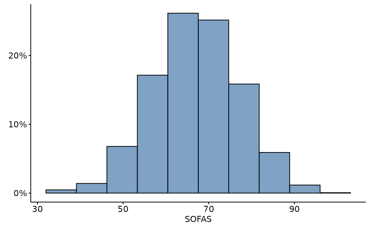
SOFAS total scores
YouthvarsSeries methods
Validate data
To explore longitudinal data we need to first use the
ratify method to ensure that Z has been
appropriately configured for methods examining datasets reporting
measures at two timepoints.
Z <- ratify(Z,
            type_1L_chr = "two_timepoints")
Inspect data
We can now specify the variables that we would like to prepare
descriptive statistics for using the renew method. The
variables to be profiled are specified in arguments beginning with
“compare_”. Use compare_ptcpn_chr to compare variables
based on whether cases reported data at one or both timepoints and
compare_by_time_chr to compare the summary statistics of
variables by timepoints, e.g at baseline and follow-up. If you wish
these comparisons to report p values, then use the
compare_ptcpn_with_test_chr and
compare_by_time_with_test_chr arguments.
Z <- renew(Z,
           compare_by_time_chr = c("d_age","d_sexual_ori_s","d_studying_working"),
           compare_by_time_with_test_chr = c("k6_total", "phq9_total", "bads_total"),
           compare_ptcpn_with_test_chr = c("k6_total", "phq9_total", "bads_total"))
The tables generated in the preceding step can be inspected using the
exhibit method.
| (N = | 1068) | (N = | 643) | p | ||
|---|---|---|---|---|---|---|
| Kessler Psychological Distress Scale (6 Dimension) | Mean (SD) | 12.153 | (5.409) | 11.069 | (5.778) | 0.001 |
| Median (Q1, Q3) | 12.000 | (8.000, 16.000) | 11.000 | (7.000, 15.000) | 0.001 | |
| Min - Max | 0.000 | 24.000 | 0.000 | 24.000 | 0.001 | |
| Missing | 0.000 | 3.000 | 0.001 | |||
| Patient Health Questionnaire | Mean (SD) | 12.632 | (6.086) | 11.194 | (6.434) | 0.000 |
| Median (Q1, Q3) | 13.000 | (8.000, 17.000) | 11.000 | (6.000, 16.000) | 0.000 | |
| Min - Max | 0.000 | 27.000 | 0.000 | 27.000 | 0.000 | |
| Missing | 1.000 | 5.000 | 0.000 | |||
| Behavioural Activation for Depression Scale | Mean (SD) | 79.814 | (26.478) | 83.571 | (25.809) | 0.010 |
| Median (Q1, Q3) | 79.000 | (62.000, 95.250) | 84.000 | (66.000, 101.000) | 0.010 | |
| Min - Max | 0.000 | 150.000 | 0.000 | 150.000 | 0.010 | |
| Missing | 1.000 | 10.000 | 0.010 |
| (N = | 1068) | (N = | 643) | ||
|---|---|---|---|---|---|
| Age | Mean (SD) | 17.555 | (3.090) | 17.770 | (3.091) |
| Median (Q1, Q3) | 17.000 | (15.000, 20.000) | 18.000 | (16.000, 20.000) | |
| Min - Max | 12.000 | 25.000 | 12.000 | 25.000 | |
| Missing | 0.000 | 0.000 | |||
| Sexual orientation | Heterosexual | 738.000 | (71.860%) | 440.000 | (71.545%) |
| Other | 289.000 | (28.140%) | 175.000 | (28.455%) | |
| Missing | 41.000 | 28.000 | |||
| Education and employment status | Not studying or working | 159.000 | (15.347%) | 152.000 | (24.398%) |
| Studying and working | 305.000 | (29.440%) | 146.000 | (23.435%) | |
| Studying only | 405.000 | (39.093%) | 167.000 | (26.806%) | |
| Working only | 167.000 | (16.120%) | 158.000 | (25.361%) | |
| Missing | 32.000 | 20.000 |
| (N = | 1068) | (N = | 643) | p | ||
|---|---|---|---|---|---|---|
| Kessler Psychological Distress Scale (6 Dimension) | Mean (SD) | 12.082 | (5.603) | 10.100 | (5.665) | 0.000 |
| Median (Q1, Q3) | 12.000 | (8.000, 16.000) | 10.000 | (6.000, 14.000) | 0.000 | |
| Min - Max | 0.000 | 24.000 | 0.000 | 24.000 | 0.000 | |
| Missing | 1.000 | 2.000 | 0.000 | |||
| Patient Health Questionnaire | Mean (SD) | 12.646 | (6.230) | 9.736 | (6.210) | 0.000 |
| Median (Q1, Q3) | 13.000 | (8.000, 17.000) | 10.000 | (5.000, 14.000) | 0.000 | |
| Min - Max | 0.000 | 27.000 | 0.000 | 27.000 | 0.000 | |
| Missing | 4.000 | 2.000 | 0.000 | |||
| Behavioural Activation for Depression Scale | Mean (SD) | 78.429 | (25.608) | 89.615 | (25.205) | 0.000 |
| Median (Q1, Q3) | 78.000 | (61.000, 95.000) | 88.000 | (73.000, 106.000) | 0.000 | |
| Min - Max | 0.000 | 150.000 | 0.000 | 150.000 | 0.000 | |
| Missing | 7.000 | 4.000 | 0.000 |
The depict method can create plots, comparing numeric
variables by timepoint.
depict(Z, x_vars_chr = c("c_sofas"), x_labels_chr = c("SOFAS"), y_labels_chr = "", z_vars_chr = "round",
       z_labels_chr = "Time", as_percent_1L_lgl = T, position_xx  ="dodge", style_1L_chr = "lancet",
       what_1L_chr = "histogram", bins=10)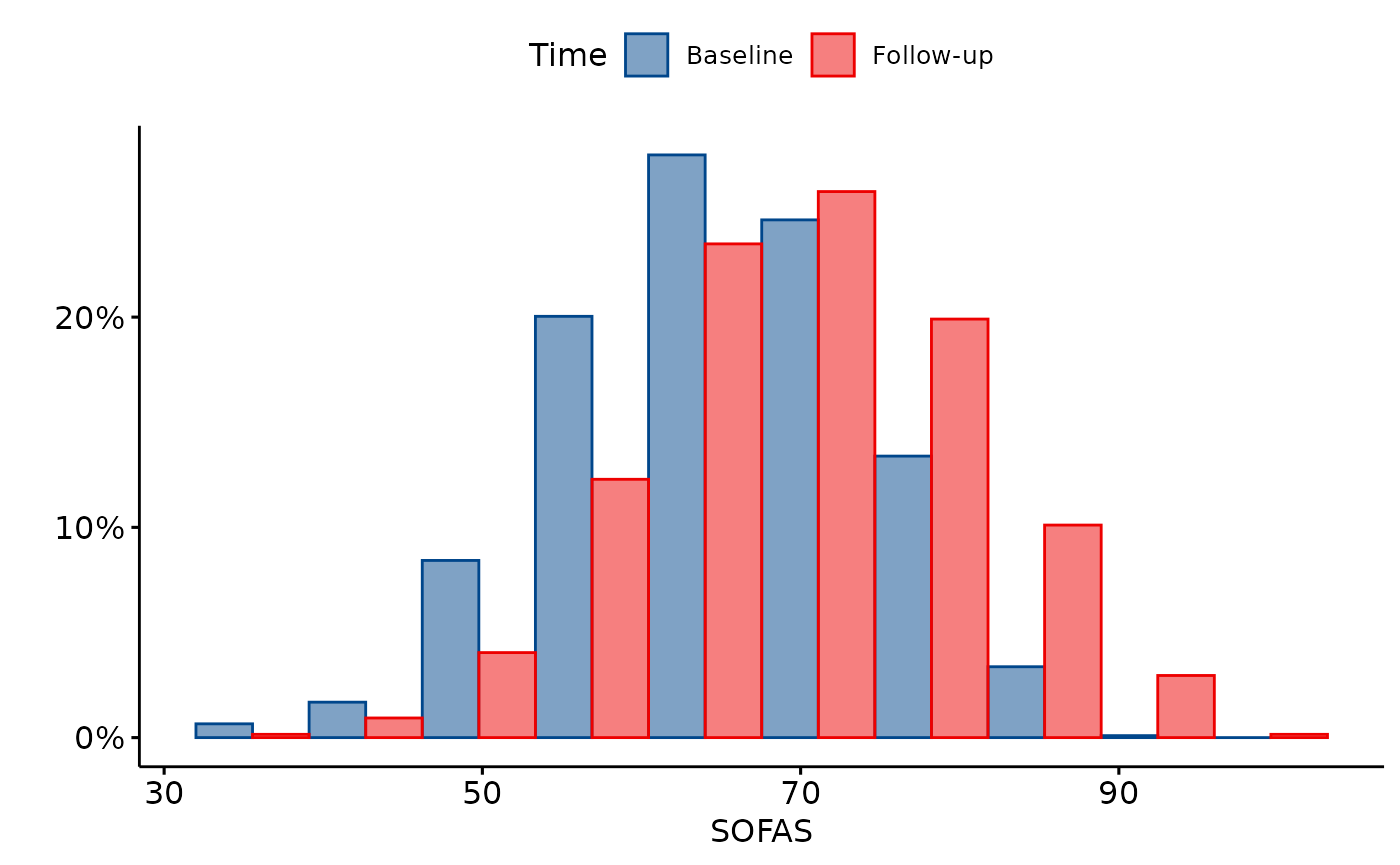
SOFAS total scores by data collection round
Share data
If and only if the dataset you are working with is
appropriate for public dissemination (e.g. is synthetic data), you can
use the following workflow for sharing it. We can share the
dataset we created for this example using the share method,
specifying the repository to which we wish to publish the dataset (and
for which we have write permissions) in a (Ready4useRepos
object).
A <- Ready4useRepos(gh_repo_1L_chr = "ready4-dev/youthvars", # Replace with your repository
                          gh_tag_1L_chr = "Documentation_0.0"), # (need write permissions).
A <- share(A,
           obj_to_share_xx = Z,
           fl_nm_1L_chr = "ymh_YouthvarsSeries")
Z is now available for download as the file
ymh_YouthvarsSeries.RDS from the “Documentation_0.0”
release of the youthvars package.